In the last lesson you learned how to create, call and operate functions. Let’s put this knowledge to use today by taking a look at how to use the function that is part of our free Value Area toolset. If you don’t have a copy installed already, I would suggest to do that now. We need the function that provides the value areas in this lesson.

Value Areas give you the areas where a defined amount of volume was traded or where price stayed in for a certain amount of time. A volume value area is the area where a certain percentage of the daily volume was traded in. While TPO (short for Time Price Opportunity) value areas are the areas where price spent a defined amount of time. You would usually look for areas with a width of about 70% of the total volume or total time (roughly one standard deviation).

In case you want to learn more about value areas, this link is a good start.

In the last session we learned that there is no need to know how a function works internally. As long as you know how to call it, you can use it.

We will make use of this, while we learn how to work with the “ABC_ValueAreas” function. This is a multiple output function and therefore it can return more than one value. As you learned in lesson six, this is done via reference inputs.

We also learned that a function should have a return value, even if it doesn’t return a result. The value areas function uses a “dummy” return value of +1 for that. This means that it just returns the value of +1 when you call the function, while all study results are returned via the “output” inputs.

You have 19 inputs in total to control and receive values from the value areas function. Since you can find a description of all the inputs in the manual of the value areas tool, let’s just briefly look at each of them here. The first seven inputs control the function and affect the results it returns. While the remaining inputs pass the function results back.

The seven inputs for configuring the function:

• StartTime  –  the time input (hhmm format) when the study should start with tracking the volume and TPO values

• EndTime  –  the time input (hhmm format) when the study should stop with the tracking

• CalcMondayToFridayOnly  –  to exclude/include weekend data

• ProfileTimeInterval –  bracket interval for each TPO in minutes

• VolumeVAPercentage –  percentage of the total volume that should fall within the volume value areas

• TPOVAPercentage  –  percentage of the TPOs that have to fall within the TPO value areas

• DynArraySize  –  size of the dynamic arrays that store the volume at each price; if you set the dynamic arrays too small, the study will raise an error

The remaining reference inputs that return the results:

• oDevelopingVolVAHigh  –  the price of the developing Volume Value Area High

• oDevelopingVolPOC  –  current developing Volume Point of Control (VPOC)

• oDevelopingVolVALow  –  current developing Volume Value Area Low

• oDevelopingTPOVAHigh  –  current developing TPO Value Area High

• oDevelopingTPOPOC  –  current developing Point of Control

• oDevelopingTPOVALow  –  current developing TPO Value Area Low

• oYesterdaysVolVAHigh  –  previous session’s Volume Value Area High

• oYesterdaysVolPOC  –  previous session’s Volume Point of Control (VPOC)

• oYesterdaysVolVALow  –  previous session’s Volume Value Area Low

• oYesterdaysTPOVAHigh  –  previous session’s TPO Value Area High

• oYesterdaysTPOPOC –  previous session’s Point of Control

• oYesterdaysTPOVALow  –  previous session’s TPO Value Area Low

All inputs that reference developing values, return the value for each bar. The reference inputs starting with oYesterdays return the final value for the previous session (as specified with the Start- and EndTime input).

Since you know what the inputs do now, you can take the next step and call the function in an indicator and plot some results.

Open PL Editor and create a new indicator (File -> New -> Indicator and click “OK”). Now choose a name you like and click “OK” again. This will bring up the new indicator.

Maybe you are like me and prefer to be able to change the function outcome easily. In that case I would suggest to create a few inputs. Start with the first seven inputs that control the function. I will stick with the same names as used in the function itself. However you are free in choosing any input name that you like. The function will work exactly the same whether or not you use the same input names.

With these default inputs the study will track value areas between 9:30 and 16:15 during the week. The value areas would have a width of 70%. This means that roughly 70% of the traded volume falls within the volume value area. In case of the TPO value area, the market spent roughly 70% of the time within the value areas. I am saying roughly, because of the way the value areas are found. Starting with the point of control the study compares the volume on the next two prices up and down from the point of control. The two prices with the higher volume will be part of the value area. This process continues until the volume within your value area is equal to or greater than 70% (depending on your input) of the session volume (or time in case of the TPO).

The default array size of 1000 is a good compromise between speed and functionality. This means that the study is able to hold the volume of 1000 price levels in each session. While this is usually more than enough, you might need a higher value in case of wide ranges. Should the study require a larger array, it will raise an error message in Multicharts. In that case you can simply raise the input value until the error disappears.

The study uses the symbol settings from the Quote Manager to compute the price of one tick. If the symbol settings are wrong, this can result in errors due to array sizes, too. Therefore I would suggest to check your symbol settings first, before you change the array input. You can find a good explanation for the QM settings here. To find the correct settings for a symbol, the exchange websites are usually a good place to look.

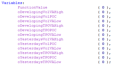
Finally we need some variables that receive and store the function outputs. You can simply use the same names as used in the input description. However you are free to use any other valid variable name. In case you need help, lesson 01 explains which variable names are valid.

With these inputs and variables, we can now call the function. When you run the indicator on the chart, the function will be computed with the inputs. The results will be passed to the variables via the reference inputs then.

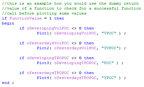
As a final step we can add some plots to display a few metrics that the function provides. We can also use the “dummy” function return value to make sure that we only plot the values if the function call was successful. As an additional check, the code checks that the plot value is not zero. This is done to avoid any scaling issues during the first bars of the chart. Otherwise a plot value of zero might compress your chart. I do this under the condition that zero is not a valid function output for my price data. Keep in mind that this might not always be the case.Therefore you should omit this check, if the data you chart can have zero as a value.

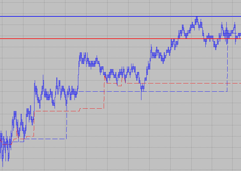
The above code will display four plots. The developing points of control for the two value areas. In addition it will show the two points of control as they were at the end of the last session. I have formatted the plots to show the last session’s values as bold line. The developing POCs are the dashed lines. The red colors are volume based values, while blue plots are TPO based results.

As a result of the lesson today, you should have an idea on how to call the function now. You can use the value areas or points of control not only in an indicator, but in other functions or even your own systems, too. One idea that comes to mind for example is to design a system that looks for virgin point of controls as entry points. This would require some programming, but the function already provides all the values that would be needed.