

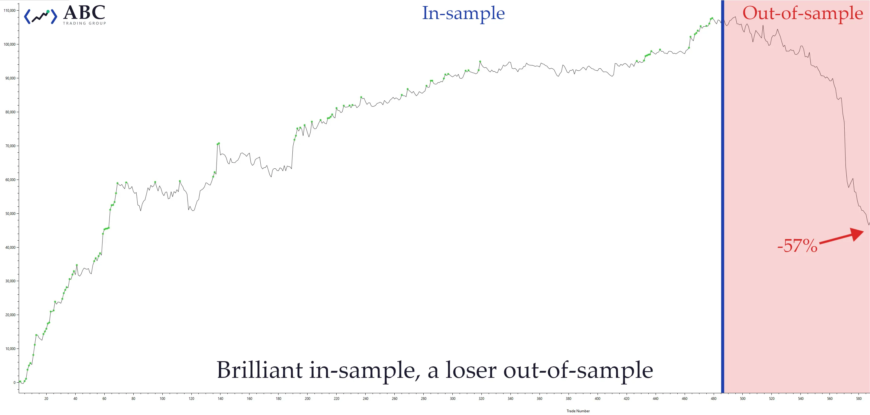
A backtest is a promise: “if you had traded this way in the past, this is what would have happened.” Many backtests break that promise without their builders ever noticing.
The strategy looks brilliant on historical data, goes live, and then bleeds money in ways the equity curve never hinted at. Here are the eight backtesting mistakes we see most often, including one subtle trap involving back-adjusted futures data that catches even experienced quants.
Key takeaways
- Most backtesting failures come from simulating a world subtly different from the real one: future information, missing losers, free execution, or guaranteed fills.
- Your universe must be point-in-time. In recent decades roughly a third to a half of the S&P 500 has turned over every ten years, so today’s constituent list is the wrong universe for almost any historical test.
- Overfitting is the silent killer: test enough parameters and something will look great by chance.
- Never compute percentage returns or cross-market ratios on difference-back-adjusted futures data. The price levels are fictitious.
- A backtest you can’t trust is worse than no backtest at all, because it gives false confidence.
Jump to a pitfall: Look-ahead bias · Survivorship bias · Overfitting · Transaction costs · Fill assumptions · Too little data · Drawdowns · Back-adjusted data
1. Look-ahead bias: trading on tomorrow’s information
Look-ahead bias means your backtest uses information that wasn’t available at the moment of the trade. It sneaks in more ways than you’d expect:
- Using today’s close to generate a signal that trades at today’s close
- Applying earnings data on the fiscal period date instead of the publication date
- Normalizing indicators with statistics computed over the entire dataset — including the future
- Using revised economic data instead of the numbers traders actually saw in real time
- Testing on today’s index constituents — an easy one to miss entirely, and the one covered below
The index constituency trap
Suppose you’re testing a momentum strategy on “the S&P 500” over the past fifteen years, and you build your universe from the current membership list. You have just handed your backtest fifteen years of hindsight about which companies would make the cut.
Every stock in that list is there because it grew large enough to be included. Tesla joined the S&P 500 before the open on December 21, 2020. By then it had risen more than 200x from its $17 IPO price. Your backtest happily buys it in 2013, a company it could not have selected at the time, chosen precisely because of what happened afterward. Every 100x story in your universe is there for the same reason. Meanwhile the companies deleted along the way (acquired, shrunk out of the index, or failed outright) never appear at all.
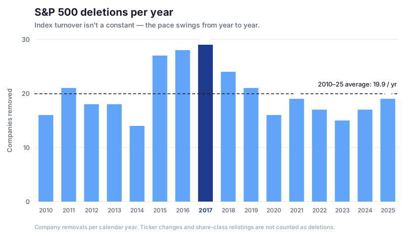
That deletion stream is much larger than most people assume. Over the past decade and a half, the S&P 500 has dropped about 20 companies a year on average, though the pace swings widely, from the mid-teens in calm years to 29 in 2017. Over a ten-year stretch that works out to over a third of the index turning over, but the rate has varied across the index’s history, so treat any figure as a snapshot of its era, not a constant. Either way, today’s membership list quietly excludes a large share of the companies your strategy would actually have held.
The same trap applies to any index-linked universe: the Russell 2000’s periodic reconstitution, the Nasdaq-100, sector and country indices, and “liquid universe” screens built from today’s volume data.
Note that this overlaps with survivorship bias (pitfall 2) but isn’t identical. Survivorship bias is about the companies that fell out of your universe going missing — and they needn’t have failed; plenty were acquired or simply dropped from the index while still trading. Constituency error is the reverse: companies that later climbed in, sitting in your universe years before they qualified. A dataset can include every departed ticker and still be wrong if the membership dates are.
The fix: enforce point-in-time discipline. Every input to a decision must have been knowable before the decision. For universes specifically, use historical constituency data with effective add and delete dates, and reconstruct index membership as of each rebalance date in the test — not once at the start.
Quick self-test: re-run your backtest with all data after a chosen date deleted from the source files, not just filtered out. If results for the earlier period change at all, something in your pipeline was reading the future.
2. Survivorship bias: only testing the winners
If your universe is “the current constituents of the S&P 500,” your backtest only trades companies that survived. The bankruptcies, delistings, and acquisitions that would have hurt you are simply missing from the data.
Enron is the canonical case, and the way it rose matters as much as the way it fell. Reinventing itself from a gas pipeline operator into an energy trader, the stock roughly quadrupled between the start of 1998 and its peak above $90 in August 2000. To any screen running in mid-2000 it looked like a buy — momentum, expanding reported earnings, index membership, analyst enthusiasm — because the accounting fraud was manufacturing the very fundamentals the screen was reading. Bankruptcy came in December 2001 and the equity went to essentially zero.
Backtest that screen on today’s constituent list and none of it happens. Enron isn’t in your universe, so the position is never taken and the loss never lands, while every stock that merely looked like Enron on the way up is still sitting there inflating your results.
The effect is usually smaller than look-ahead bias, but it is concentrated exactly where people go looking for edge: small caps, emerging markets, and any value or distress screen, where failure rates are highest. Hedge fund and mutual fund databases have the same problem: closed funds stop reporting, so index-of-fund returns are quietly biased upward.
The defense: the same discipline as before. Use point-in-time universes and datasets that keep dead tickers and delisted contracts with their final returns. Worth checking that your vendor actually retains them, because plenty quietly drop them.
3. Overfitting and data snooping
Test enough parameter combinations and one of them will look spectacular by pure chance. A moving-average crossover with lookbacks of 13 and 47 that beats every other combination is almost certainly noise, not signal.
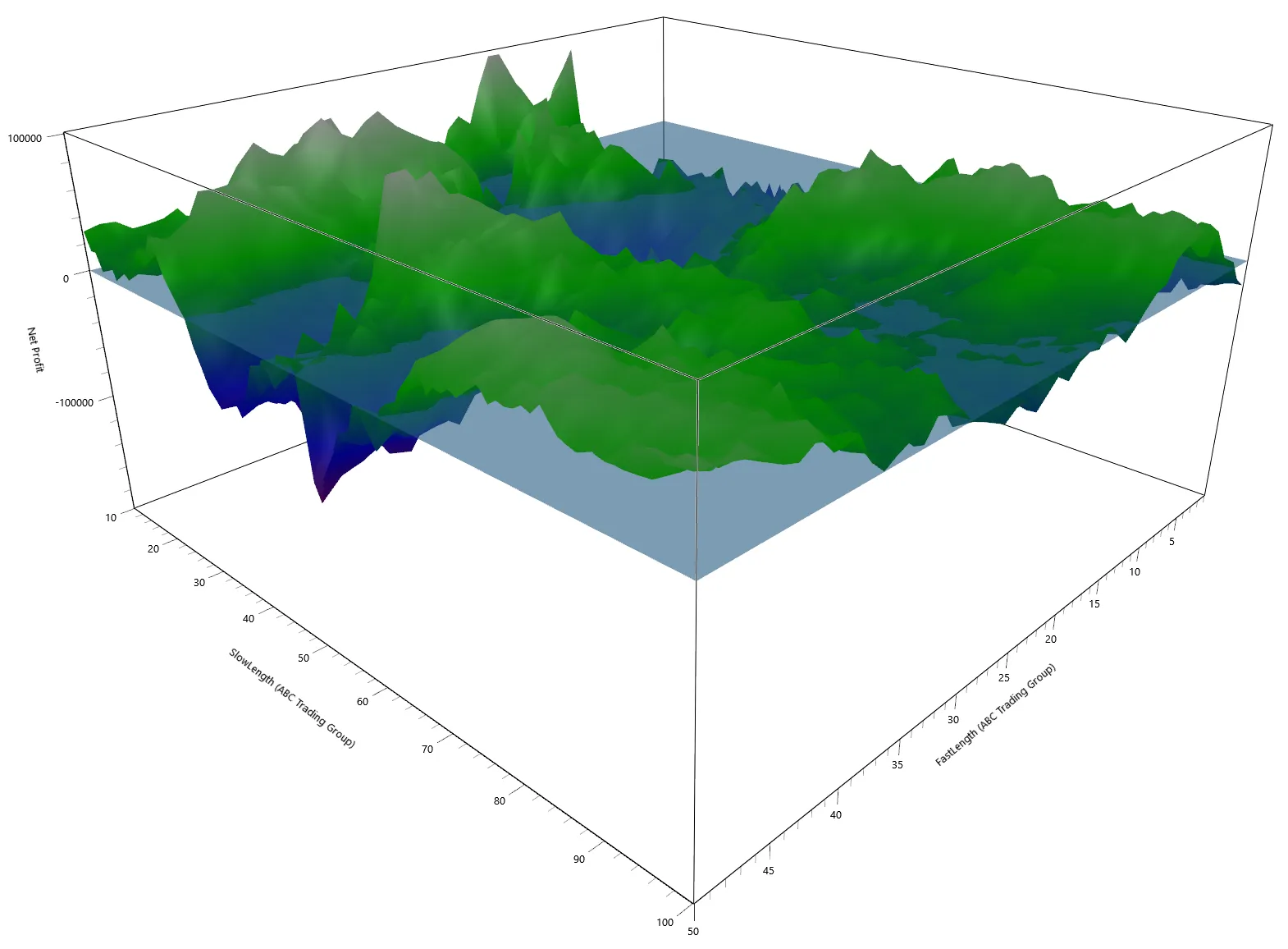
The arithmetic here is what gets people. Run 1,000 random strategies against the same history and roughly 50 will clear a 95% significance bar without any edge at all. Report only the best of them and you have a beautiful, meaningless equity curve.
Related sins: repeatedly “peeking” at your out-of-sample data until it effectively becomes in-sample, and reporting only the best of dozens of strategy variants.
The fix: fewer parameters, economically motivated rules, walk-forward testing, and deep skepticism toward anything that collapses when a parameter moves slightly. Track how many variants you tested and discount the result accordingly. The more combinations you tried, the higher the bar the winner has to clear before you believe it. A robust parameter sits on a plateau, not a spike: if 13/47 works and 12/45 doesn’t, you found noise.
4. Ignoring transaction costs and slippage
Commissions are the smallest part of the problem. Crossing the bid-ask spread, slippage in fast markets, and the price impact of your own size can turn a profitable high-turnover backtest into a losing live strategy.
Consider a strategy that turns over its book daily and earns 8 basis points per trade before costs. On a $40 stock, crossing a one-cent spread round-trip costs about 2.5 bp, and a little slippage on top takes you to roughly 4 bp — half that edge, gone before you account for anything else. Add market impact at any real size and the strategy is flat to negative. Nothing about the pre-cost backtest warned you.
This bites hardest exactly where naive backtests look best: short holding periods, illiquid instruments, and thin contracts.
In practice: model costs pessimistically, then stress-test with them doubled. It’s also worth capping position size at a small fraction of historical average volume and re-running: if the returns depend on trading 20% of a day’s volume, the backtest is fiction.
5. Unrealistic fill assumptions
Backtests love to assume perfect fills. Reality usually doesn’t.
- Limit orders: a touch of your price doesn’t guarantee execution — you may be far back in the queue, so count a fill only when the market trades through your level.
- Stop orders: a stop fills at the next available price, not your trigger — in fast markets, meaningfully worse.
- Auction prices: you can join the opening or closing auction, but the open or close in your data isn’t necessarily the auction price, and your own size — especially in thin names — moves the print.
- Overnight gaps: a gap can leap clean past your stop. A stop at 95 on a stock that closes at 100 and reopens at 82 will likely fill near 82, not 95.
The fix: model conservative slippage and worse-than-ideal fills. If the edge disappears, it probably wasn’t real.
6. Too little data, too few market regimes
A strategy tested only on 2020–2025 has never seen a decade of sideways markets or a liquidity crisis it wasn’t shaped by. Trend-following looks unbeatable if you only test trending years.
The reverse is just as common: a short-volatility strategy backtested through 2017 looked like free money right up until February 2018, when a single volatility spike erased years of steady gains in days. The backtest wasn’t wrong about the past; it simply ended just before the event that defines the strategy’s risk.
What to test: bull, bear, sideways, high-volatility and low-volatility regimes. Treat performance in a regime you haven’t seen as unknown rather than implied.
7. Ignoring the path: drawdowns and risk of ruin
A backtest that reports only final CAGR hides the 55% drawdown in the middle — the one that would have forced you (or your investors) out long before the recovery. A subtler version of the same mistake is assuming a capital path you could never have survived, compounding smoothly through the drawdown with no margin call, redemption, or forced liquidation at the bottom.
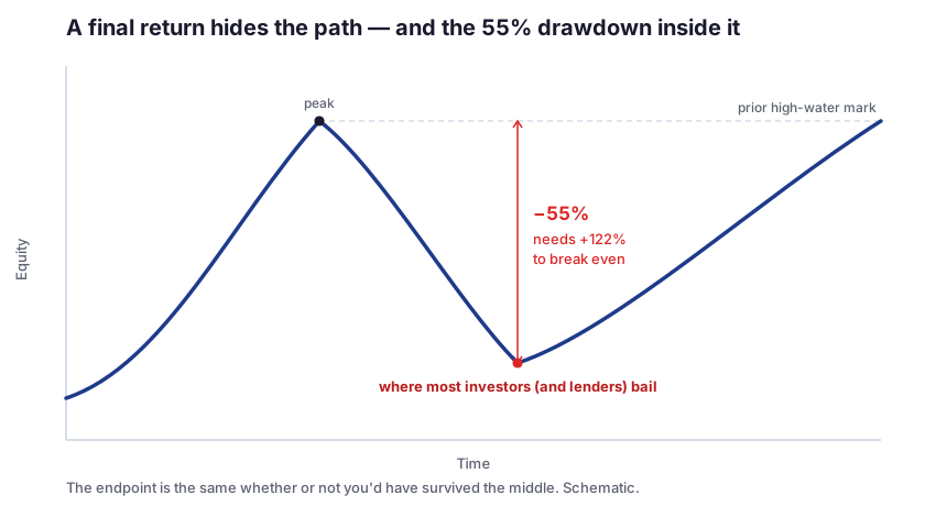
A 55% drawdown requires a 122% gain just to break even. If it takes three years to recover, the question isn’t whether the strategy was profitable. It’s whether you, or your capital, would still have been there.
The fix: evaluate maximum drawdown and drawdown duration, and ask honestly whether you would have kept trading through the worst stretch.
8. Computing ratios and percentage returns on back-adjusted data
This pitfall deserves special attention, because here the data itself is the trap.
Why back-adjusted futures prices are fictitious
Futures contracts expire, so continuous price histories are built by stitching contracts together. The most common method is back-adjustment: at each roll, the gap between old and new contract is subtracted from the entire prior history, removing artificial jumps at roll dates.
That’s exactly right for point-based P&L: day-to-day differences in a back-adjusted series correctly reflect what a position gained or lost.
But the price levels are fictitious. Years of accumulated roll adjustments shift the earlier history by a large, method-dependent amount, and the direction depends on the market’s curve — contango pushes the past up, backwardation pulls it down. WTI crude shows it plainly: a continuous series anchored to today puts crude near $152 in early 2006, when it actually traded around $61, and peaks near $217 in 2008 — above crude’s real all-time high of about $147. Crude did famously settle at −$37 for a single day in April 2020, but front-month prices were back in the $30s within weeks; the back-adjusted series, by contrast, stays negative for months. That persistence is the artifact. Only the day-to-day differences are real; the levels are not.
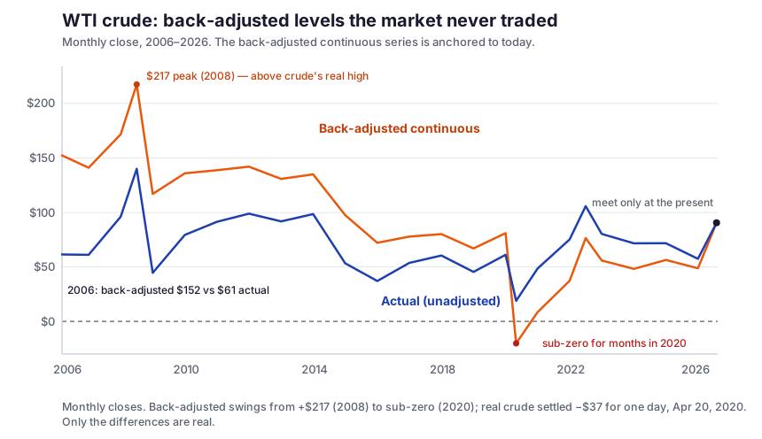
What goes wrong when you divide by a fictitious price
- Percentage returns. A $5 move on crude trading near $36 in October 2020 was a 14% move. Measured against that month’s back-adjusted level of about −$4, the same $5 swings to roughly −125% — a bigger, sign-flipped number from identical dollars. Near zero the percentage explodes toward infinity, and below zero it inverts. Your volatility estimates, Sharpe ratios, and compounded equity curves all inherit those distortions.
- Ratios between markets. Spread strategies built on the ratio of two back-adjusted series (gold/silver, cross-market pairs) are dividing two fictitious levels, each shifted by its own roll history. The resulting ratio’s level, trend, and mean-reversion behavior are arithmetic artifacts, not the market.
- Percentage-based stops and position sizing. A “2% stop” or capital-divided-by-price sizing uses the distorted level, so early-history trades are sized and stopped nothing like reality: positions balloon when the level sits near zero and shrink when it’s inflated, and neither resembles the size you’d actually have traded.
The insidious part: nothing crashes. The backtest runs, the numbers look plausible, and the distortion is worst in the oldest data, where you’re least likely to spot-check.
Which series to use for which calculation
| You are computing | Use this series |
|---|---|
| Point or dollar P&L | Back-adjusted (difference) |
| Percentage returns, volatility, Sharpe | Ratio-adjusted (or the unadjusted contract held) |
| Cross-market ratios and spreads | Unadjusted (actual contract prices) |
| Percentage stops and position sizing | Unadjusted price of the contract held |
| Chart levels, support and resistance | Unadjusted |
How to handle back-adjusted data correctly
- Use point (difference-based) calculations on back-adjusted series. That’s what they’re built for.
- For percentage returns, use a ratio-adjusted (proportionally adjusted) series — which multiplies rather than subtracts at each roll — or compute each day’s return against the actual unadjusted price of the contract held that day.
- Build cross-market ratios from unadjusted (actual contract) prices. Ratio-adjusting each leg doesn’t fix it: the two legs carry different roll factors, so the ratio’s history stays distorted.
- Sanity check: scan your series for zero or negative prices, and for early-history returns that are much larger than recent ones. The first is a near-certain sign of a distorted level. The second is a red flag, not proof: it can also reflect a genuinely volatile early regime, so check whether those large returns coincide with a near-zero price level before blaming the data.
A pre-flight checklist
Before you trust any backtest, confirm you can answer yes to each of these:
- Every input was knowable before the decision that used it
- The universe is reconstructed from point-in-time index constituency at each rebalance
- Delisted, acquired, and bankrupt securities are present in the data
- The edge holds after penalizing for how many variants you tested
- Costs and slippage are modeled pessimistically, then doubled as a stress test
- Fills assume worse-than-ideal execution, and gaps are handled explicitly
- The test spans multiple regimes including at least one crisis
- Maximum drawdown and its duration are reported alongside returns
- Percentage and ratio math is never run on difference-back-adjusted prices
Any item you can’t answer yes to is a reason to keep the strategy on paper a while longer. If you would rather have someone else run that list against your code, that is what independent strategy validation is for.
The common thread
Every pitfall above is the same mistake in different clothing: the backtest simulates a world subtly different from the one you’d actually trade in — a world with tomorrow’s information, no dead companies, index membership you couldn’t have known, free execution, guaranteed fills, or prices that never existed.
The goal of a backtest isn’t a beautiful equity curve. It’s an honest answer. Build your process so that when the backtest looks great, you can trust it — and when it looks mediocre, you found out for the price of CPU time instead of capital.
Our trading-system case studies show what that testing looks like on the projects clients bring us.
Frequently asked questions
What is the most common backtesting mistake?
Overfitting. Testing many parameter combinations and keeping the best one almost guarantees you’ve fit noise rather than signal. Look-ahead bias is a close second because it’s so easy to introduce accidentally.
Why does index constituency matter in a backtest?
Because index membership changes constantly, and companies are added only after they’ve already performed well. Over the past decade and a half the S&P 500 has dropped about 20 companies a year on average, enough that over a third of the index turns over in a ten-year window, though the rate has varied widely across history and by period. Test on today’s membership list and you’ve quietly excluded a large share of the companies your strategy would actually have held. You need historical constituency data with effective add and delete dates, applied as of each rebalance date.
What is point-in-time data?
Data as it existed and was known on a given historical date: unrevised economic figures, as-first-reported fundamentals, and the index membership actually in force that day. It is one of the most effective defenses against look-ahead bias.
Can I use back-adjusted futures data for backtesting?
Yes — for point-based (dollar or tick) P&L, back-adjusted data is the right choice. Just don’t compute percentage returns, ratios, or percentage-based sizing from its price levels, because those levels are artifacts of the adjustment process.
What’s the difference between back-adjusted and ratio-adjusted futures data?
Back-adjustment subtracts the roll gap from prior history, preserving point differences but distorting levels and percentages. Ratio adjustment multiplies prior history by the roll ratio, preserving percentage changes but distorting point differences. Pick the one that matches the math you’re doing.
How much historical data do I need for a reliable backtest?
Enough to cover multiple distinct market regimes — ideally 10–20+ years for daily strategies. More important than raw length is regime diversity: bull, bear, sideways, and at least one crisis period.
This post is for educational purposes and does not constitute investment advice. Past performance — even honestly backtested past performance — is no guarantee of future results. See our risk disclaimer for the full statement on hypothetical and simulated performance.