

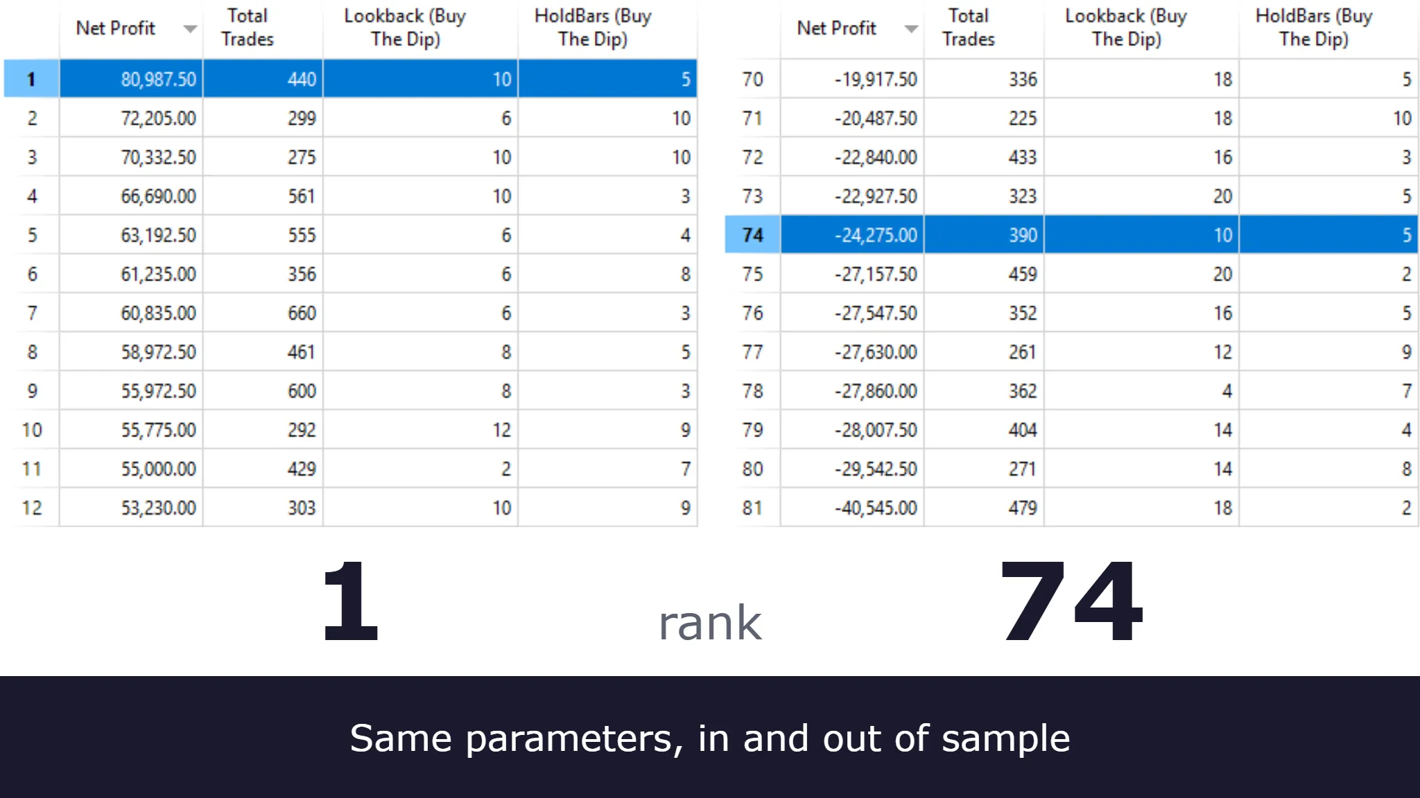
An optimizer scores every parameter set by the metric you chose, and one of them comes out on top. Where that set ranks on the data it was chosen from can tell you surprisingly little about where it will rank on data it has never seen.
A top-ranked set exists whether or not the history contains anything worth finding. So the useful question about that set is not how good it looks but what put it there: a pattern that repeats, or luck particular to the stretch of history it was tested on. Nothing in this article can prove the first. What the checks below can do is flag signs that a strategy is overfit, meaning it is tuned to noise in its test history instead of to a pattern that repeats.
Key takeaways
- An optimization report always has a top row, even when the rule has no edge. Each row’s result combines any true edge with luck specific to the tested history, so after sorting, the top row often reflects more luck than the others.
- In our example, the in-sample winner out of 100 parameter pairs ranked 74th out of sample, and the two rankings were essentially uncorrelated. Market conditions also changed between the two periods, and the example cannot separate that from luck.
- The optimizer counts its own passes. No report counts the filters, sessions, instruments, and start dates tried by hand, yet each of those is a variant tried too.
- Judge a parameter set by its neighbors, not by itself. A winner that stands well clear of everything around it deserves suspicion, not confidence.
- A large trade count does not settle anything on its own. Remove the best trades to see how much of the result rests on them.
- Out-of-sample data gives one honest reading. Once the rules change after you have seen the results, the data is no longer out of sample.
- None of these checks can show that a strategy is sound. They can only show that a result is fragile.
Jump to: The example · Why the top row misleads · Variants no report counts · Neighbors · Trade counts · Out-of-sample data · Walk-forward · Checklist
The example in this article
Every number below comes from one example: a short-term mean-reversion strategy on the E-mini S&P 500, optimized on one stretch of history, with all 100 parameter pairs then run unchanged on the next.
The rules are deliberately plain. When the daily close is the lowest close of the last Lookback bars, buy at the next open. When it is the highest, sell short at the next open. Exit at the next open once HoldBars bars have closed after the entry bar. No new signal is taken while a position is open. In EasyLanguage:
Inputs:
    Lookback            ( 10 ),
    HoldBars            ( 5 );

Variables:
    lowestClose         ( 0 ),
    highestClose        ( 0 );

lowestClose = Lowest( Close, Lookback ) ;
highestClose = Highest( Close, Lookback ) ;

if MarketPosition = 0 then begin
    // At short Lookbacks, unchanged closes can be both lowest and highest;
    // the second condition keeps such a bar from signaling long and short at once
    if Close = lowestClose and Close < highestClose then
        Buy ( "Long" ) next bar at market ;
    if Close = highestClose and Close > lowestClose then
        SellShort ( "Short" ) next bar at market ;
end ;

if MarketPosition = 1 and BarsSinceEntry >= HoldBars then
    Sell ( "LX" ) next bar at market ;

if MarketPosition = -1 and BarsSinceEntry >= HoldBars then
    BuyToCover ( "SX" ) next bar at market ;
The optimization tried Lookback from 2 to 20 in steps of 2 and HoldBars from 1 to 10, for 100 parameter pairs. We ran it in MultiCharts on daily bars of IQFeed’s back-adjusted continuous E-mini S&P 500 contract (@ES#C), trading one contract and charging $55 per round turn for commission and slippage. The in-sample period runs from October 7, 1997 through December 31, 2012, and the out-of-sample period from January 2, 2013, through September 11, 2026. All results are dollar P&L, because back-adjusted data preserves dollar differences but distorts percentages.
Two simplifications are worth stating. A flat $55, two ticks of slippage per side plus $5 for commission and fees, is probably optimistic for the thinner early years of the E-mini contract, and the cost of rolling from one contract to the next is not simulated. The strategy was chosen because it shows the effect clearly, and it is not a recommendation to trade.
Why the top row of an optimization report misleads
Every row in an optimization report combines two things: any true edge the rule has in that market, and luck particular to the history the test ran on. Sorting by result cannot separate them. The rows at the top are there partly because their luck was good, and that luck does not carry into the next stretch of history. So the winner tends to fall back out of sample even when the rule has a true edge, and the more rows the sort had to choose from, the more luck the top row tends to carry. Statisticians call this a form of selection bias.
In the example, the in-sample optimization looked encouraging. Ninety of the 100 pairs were profitable, and the best, Lookback 10 with HoldBars 5, made $80,987.50 on 440 trades. Out of sample, the same pair lost $24,275 on 390 trades and ranked 74th of 100.
The rest of the in-sample top ten fared better, but not in the way their ranks suggested. Seven of them were still profitable out of sample, yet only one made the out-of-sample top ten. The out-of-sample winner, Lookback 4 with HoldBars 6, had ranked 35th in sample. Across all 100 pairs, the Spearman rank correlation between in-sample and out-of-sample net profit was −0.03. In this example, knowing where a pair ranked in sample told you essentially nothing about where it would rank out of sample. Costs do not explain this: before the $55 per round turn, the in-sample winner lost $2,825 out of sample and ranked 73rd, and the rank correlation was 0.06.
The in-sample and out-of-sample periods differ in character. On the back-adjusted series the test ran on, the first gained about 200 points from start to finish and the second about 5,500, rising for most of its length. So the in-sample winner may have fallen partly because market conditions changed, not only because its in-sample luck did not repeat. In sample, its long trades made $39,777.50 and its short trades $41,210. Out of sample, its long trades made $111,922.50 and its short trades lost $136,197.50. The example cannot say how much of the fall was luck and how much was the change in market conditions.
Notice what did not happen. Profits did not disappear across the grid. Fifty-eight of the 100 pairs were still profitable out of sample, but the profit came from the long side: longs made money in every pair and shorts lost money in every pair. What failed to carry over was the ranking.
The variants no report counts
The platform’s optimizer counts its passes, 100 in the example. It does not count the ones that happened before it was opened. A filter added after looking at the equity curve. A session window moved by half an hour. The instrument or timeframe that “worked better.” The start date of the test. The rule that was dropped because results improved without it. Each of those is a choice that was tried and then set, and none of them appears in any report.
That matters because the selection effect grows with the number of things tried, not with the number the platform counted. A report showing 100 passes can sit on top of hundreds of untracked ones, and the winner carries the luck of all of them.
Developing a strategy with an AI assistant runs the same loop, only faster. Ask for an improvement, run the backtest, paste the results back, and ask again. Each round is an optimization pass, except that nothing in the loop keeps count. The same thing happens by hand, just more slowly.
None of this limits what an assistant can build. It can write a walk-forward harness or parameter sweep, though what it produces needs checking like any other code before you rely on it. What no tool can supply afterward is a reliable count of how many variants were tried on the way to the version in front of you, including the changes made outside any conversation. That count is reliable only if someone kept it from the start.
What to keep: a variant log, started at the first backtest, recording the date, what changed, and the result. It is dull, but without it you cannot know how heavily to discount the winner for the number of variants behind it.
Formal tests need more than the variant log holds. White’s Reality Check needs each variant’s full return series. The Deflated Sharpe Ratio needs each variant’s Sharpe ratio, which it uses to adjust the winner’s Sharpe for how many variants were tried.
Judge a parameter set by its neighbors
A single cell in an optimization grid is one measurement with luck attached. The cells around it were tested on the same data with slightly different settings, so they show how much of the result depends on the exact values chosen.
Two questions do most of the work. What share of the neighbors are profitable? And how far does the result fall one step away in each direction? A set whose neighbors are mostly profitable and not far below it is at least not balanced on a knife-edge. A set that stands well clear of everything around it has a result that depends on its exact values, and a result that depends on exact values is the kind luck can produce.
Include the diagonal neighbors, where both parameters change at once, and look further out when the grid steps are small. Checking only the four neighbors along the axes misses interactions. Two changes that each look harmless alone can do damage together, and those four never test the combination. Choosing a set because its whole region is profitable is also a different decision from choosing it because it tops the list, even when both land on the same cell.
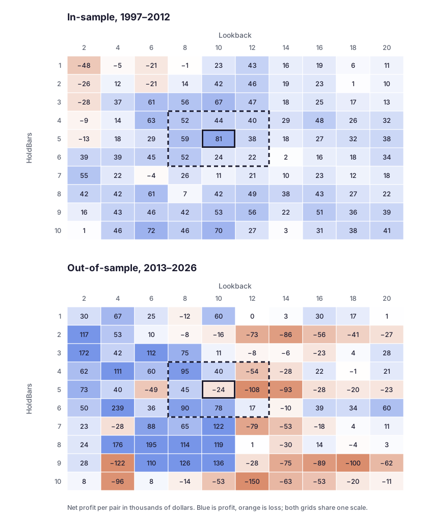
In the example, the in-sample winner stood clearly above its eight neighbors. They made between $22,290 and $58,972.50, so the winner’s $80,987.50 was $22,015 above the best neighbor. All eight neighbors were profitable, which looks reassuring, but the gap was a warning: nothing next to the winner came close to its result.
Out of sample, six of the eight neighbors stayed profitable while the winner itself lost money.
That is not an argument for picking by neighborhood instead. The neighbor at Lookback 12 and HoldBars 5 lost $108,190 out of sample. A neighborhood check can flag a result that depends on its exact values. It cannot tell you whether a set will remain profitable out of sample.
How many trades a result rests on
No trade count makes a result trustworthy. Any rule of thumb that names one is a convention, not a finding. What matters more is how many choices went into the result. Every parameter in the grid, and every choice made outside the optimizer, gives luck one more way in. The more choices, the more trades the result needs before its average means much.
A trade count also says nothing about how the profit is distributed, but that is easy to check. Take the trade list, remove the best few trades, and recompute. The fewer trades it takes to erase the profit, the more fragile the result.
The example’s in-sample winner produced 440 trades, a count that looks comfortable. Its trade list tells a different story:
| Trades included | In-sample net profit |
|---|---|
| All 440 | $80,987.50 |
| Without the best 5 | $53,837.50 |
| Without the best 10 | $33,650.00 |
| Without the best 20 | −$287.50 |
Twenty trades, under 5% of the total, account for the entire in-sample profit. That was not peculiar to the winner. Without their best 20 trades, 89 of the 90 profitable pairs lost money in sample, and so did the out-of-sample winner over 2013 to 2026. Eight of the in-sample winner’s ten most profitable trades were entered during the selloffs of 2000 to 2002, 2008, and 2011. A result concentrated in a few episodes is not necessarily noise. But it depends on those episodes, and whether the next stretch of history contains episodes like them is something the backtest cannot tell you.
Out-of-sample data can only be used once
Holding data back gives you one honest reading of how the rules behave on history they were not fitted to. The reading is honest only once. If you look at the out-of-sample result, change a rule, and look again, the second look is no longer out of sample. The change was informed by that data, so the data now counts as in sample.
Three habits keep the reading honest:
- Decide the split before the first run, and write it down. The example split its history at the end of 2012, close to the middle, so both halves had a long run of trades and each contained severe selloffs: 2000 to 2002 and 2008 in the first half, 2020 and 2022 in the second.
- Record the date of the first out-of-sample look. After any rule change made past that date, treat the data as used.
- Know where the next reading comes from. Once the holdout has been used, the options are a period or a related instrument that played no part in developing the rules, or forward testing on live data.
Walk-forward testing: what it tests and what it does not
Walk-forward testing repeats the optimize-then-test cycle across history. It optimizes on one window, trades the following window with the winning parameters, moves both windows forward, and stitches the out-of-sample pieces together.
It answers whether re-optimizing on a schedule and trading the resulting parameters would have worked over the history you have. That is a different question from whether today’s best parameters are good, and reading a walk-forward result as an answer to the second question is the misreading to avoid.
Windows come in two kinds. Anchored windows keep the start date fixed and grow, so each optimization sees all the history up to that point. Rolling windows keep a fixed length and move, so older data drops out. Rolling windows respond faster to change but give each optimization less data to work with. Anchored windows grow steadier as history accumulates, but also slower to notice that anything has changed.
Read the parameter path, not only the stitched equity curve. If the winning values jump across the grid from one window to the next, the optimizer may be fitting noise, even when the combined curve looks acceptable. A single lasting shift can reflect a change in market conditions. Values that keep jumping back and forth are harder to explain that way. Jumps between values that perform about the same matter less.
What walk-forward testing cannot catch:
- A market condition absent from the whole dataset. Every window inherits the same blind spot, the problem our backtesting article covers under too few market regimes.
- Costs modeled too optimistically. Every window uses the same cost model, so the error repeats in each one.
- The untracked variants from earlier in this article. Walk-forward counts its own optimizations and nothing that happened before it was set up.
In-sample length, out-of-sample length, step size, anchored versus rolling, and the objective function are all parameters, and tuning them until the stitched curve looks right is a second optimization layer on top of the first. They belong in the variant log too.
Platforms differ widely in how they run walk-forward tests and what they report, so this section stays with the method rather than any one tool.
Before you trade it
- The split between in-sample and out-of-sample data was fixed before the first run
- The date of the first out-of-sample look is recorded
- A variant log records every change tried, including the ones made outside the optimizer
- The region around the chosen set was inspected, including the diagonals
- The result was recomputed with its best trades removed, to see how much of it rests on them
- The in-sample winner’s out-of-sample rank was checked, not only its profit
- A walk-forward run’s parameter path was read, not only its equity curve
What these checks can and cannot tell you
Every check in this article can show that a result is fragile. None of them can show that it is sound. The example’s winner showed a warning sign before any out-of-sample data was touched: a wide gap to its neighbors. Across the grid, such gaps did not predict how pairs did out of sample, so the gap is only a reason for doubt. A parameter set that passes every check has not been proven; it has only survived the tests you ran.
That asymmetry is not a reason to skip the checks. It is the reason to run them before the market runs them for you. If you want your own strategy put through them, our strategy validation service runs out-of-sample, walk-forward, and parameter-sensitivity testing and reports what the evidence does and does not support.
Frequently asked questions
Does optimizing a strategy always overfit it?
No. Optimization is a search, and searching is not the problem. The problem is treating the best result of the search as an estimate of what comes next. The more combinations the search tried, and the more choices were made outside it, the more of the winner’s result is likely to be luck. The checks in this article are ways of looking for it.
How much data should I hold out?
There is no standard fraction. The held-out period needs to be long enough for each parameter set to produce a meaningful number of trades. The example in this article split its history close to the middle, which gave both halves a long run of trades and severe selloffs. That was a choice for this example, not a rule.
Is walk-forward testing enough on its own?
No. It tests whether a re-optimization procedure would have worked, and it inherits the blind spots of the data and the cost model it runs on. It also cannot see the variants tried before it was set up. It belongs alongside the other checks, not in place of them.
How many trades does a backtest need?
There is no fixed number. The count a result needs grows with the number of choices that went into it, including the ones no report records. And a large count is not enough by itself. In this article’s example, 440 in-sample trades looked ample, yet the best 20 of them accounted for the whole profit. Check how the profit is distributed, not only how many trades produced it.
Are strategies developed with AI tools more prone to overfitting?
Not in kind: overfitting works the same way whether the changes come from you or from an assistant. Every change made after seeing a result is another variant tried. What differs is speed. An assistant makes it easy to run many rounds of “improve, backtest, repeat” in an afternoon, and nothing in that loop keeps count. A variant log closes that gap, regardless of how the strategy is built.
This post is for educational purposes and is not trading advice. The strategy in it is an illustration, and its results are hypothetical. See our risk disclaimer for the full statement on simulated performance.